This tutorial explains how to save a chart as an png image file using R.
Have you generated a chart in R which you want to save as an image, simply for posterity or because you want to use in a document or presentation?
For an example, we can use the example data set faithful in the MASS package to produce plot via plot():
library(MASS)
plot(faithful)
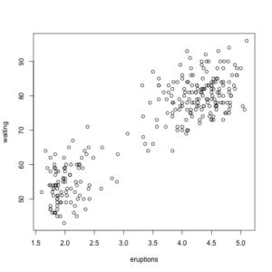
This is just a sample dataset built into R, and the above code produces a scatter plot of the waiting time against duration of eruptions by the Old Faithful Geyser.
The solution
We’ll look to save our chart to a PNG file. We do this by calling png(file="faithful.png") beforehand, where faithful.png is the file I want it to save to, and graphics.off() after.
library(MASS)
png(file="faithful.png")
plot(faithful)
graphics.off()
This gives the following file:

That’s it – the png() function tells r to start creating the a PNG file, and graphics.off() closes and saves the file. The chart produced by the plot() command between those lines is output to the specified PNG file.
We’ve used plot() but its worth noting that this will work identically for most other chart functions, such as hist() which produces histograms.
Output Location
This code saves the file to your current working folder in R. You can see what this is by typing the getwd() function in R.
If you want the output elsewhere, you can change the working directory using the setwd() function, for example the following will set the working directory to C:/Temp/ on a Windows computer (assuming that folder has already been created), before saving the chart there. Note that R requires forward slashes in the folder path, rather than backslashes:
setwd("C:/Temp/")

library(MASS)
png(file="faithful.png")
plot(faithful)
graphics.off()
Alternatively, you can specify the full path to where the file should be saved:
library(MASS)
png(file="C:/Temp/faithful.png")
plot(faithful)
graphics.off()
Save as other file types
R supports different filetypes – the following functions exist, and work in a similar way to the png() one we used above.
png()– PNG filesjpeg()– JPEG (.jpg or .jpeg) filebmp()– Bitmap (.bmp) filestiff()– TIFF files
It’s also useful sometimes to change the width and height of the chart produced, or set the background to transparent. This is done by passing arguments to the png() function, for example:
library(MASS)
png(file="faithful.png", width=300, height=250, bg="transparent")
plot(faithful)
graphics.off()